[1]:
import numpy as np
import pandas as pd
import matplotlib.pyplot as plt
from sklearn.model_selection import train_test_split
from sklearn.model_selection import StratifiedShuffleSplit
Project Goals
To create a model that predicts median house values in Californian districts, given a number of features from these districts
Get the data
[125]:
file_name = 'data/raw/housing.csv'
housing_df = pd.read_csv(file_name)
housing_df.head()
[125]:
| longitude | latitude | housing_median_age | total_rooms | total_bedrooms | population | households | median_income | median_house_value | ocean_proximity | |
|---|---|---|---|---|---|---|---|---|---|---|
| 0 | -122.23 | 37.88 | 41.0 | 880.0 | 129.0 | 322.0 | 126.0 | 8.3252 | 452600.0 | NEAR BAY |
| 1 | -122.22 | 37.86 | 21.0 | 7099.0 | 1106.0 | 2401.0 | 1138.0 | 8.3014 | 358500.0 | NEAR BAY |
| 2 | -122.24 | 37.85 | 52.0 | 1467.0 | 190.0 | 496.0 | 177.0 | 7.2574 | 352100.0 | NEAR BAY |
| 3 | -122.25 | 37.85 | 52.0 | 1274.0 | 235.0 | 558.0 | 219.0 | 5.6431 | 341300.0 | NEAR BAY |
| 4 | -122.25 | 37.85 | 52.0 | 1627.0 | 280.0 | 565.0 | 259.0 | 3.8462 | 342200.0 | NEAR BAY |
[126]:
housing_df.info()
<class 'pandas.core.frame.DataFrame'>
RangeIndex: 20640 entries, 0 to 20639
Data columns (total 10 columns):
longitude             20640 non-null float64
latitude              20640 non-null float64
housing_median_age    20640 non-null float64
total_rooms           20640 non-null float64
total_bedrooms        20433 non-null float64
population            20640 non-null float64
households            20640 non-null float64
median_income         20640 non-null float64
median_house_value    20640 non-null float64
ocean_proximity       20640 non-null object
dtypes: float64(9), object(1)
memory usage: 1.6+ MB
[4]:
housing_df['ocean_proximity'].value_counts()
[4]:
<1H OCEAN     9136
INLAND        6551
NEAR OCEAN    2658
NEAR BAY      2290
ISLAND           5
Name: ocean_proximity, dtype: int64
[5]:
housing_df.describe()
[5]:
| longitude | latitude | housing_median_age | total_rooms | total_bedrooms | population | households | median_income | median_house_value | |
|---|---|---|---|---|---|---|---|---|---|
| count | 20640.000000 | 20640.000000 | 20640.000000 | 20640.000000 | 20433.000000 | 20640.000000 | 20640.000000 | 20640.000000 | 20640.000000 |
| mean | -119.569704 | 35.631861 | 28.639486 | 2635.763081 | 537.870553 | 1425.476744 | 499.539680 | 3.870671 | 206855.816909 |
| std | 2.003532 | 2.135952 | 12.585558 | 2181.615252 | 421.385070 | 1132.462122 | 382.329753 | 1.899822 | 115395.615874 |
| min | -124.350000 | 32.540000 | 1.000000 | 2.000000 | 1.000000 | 3.000000 | 1.000000 | 0.499900 | 14999.000000 |
| 25% | -121.800000 | 33.930000 | 18.000000 | 1447.750000 | 296.000000 | 787.000000 | 280.000000 | 2.563400 | 119600.000000 |
| 50% | -118.490000 | 34.260000 | 29.000000 | 2127.000000 | 435.000000 | 1166.000000 | 409.000000 | 3.534800 | 179700.000000 |
| 75% | -118.010000 | 37.710000 | 37.000000 | 3148.000000 | 647.000000 | 1725.000000 | 605.000000 | 4.743250 | 264725.000000 |
| max | -114.310000 | 41.950000 | 52.000000 | 39320.000000 | 6445.000000 | 35682.000000 | 6082.000000 | 15.000100 | 500001.000000 |
[6]:
housing_df.hist(bins=50, figsize=(20,15));
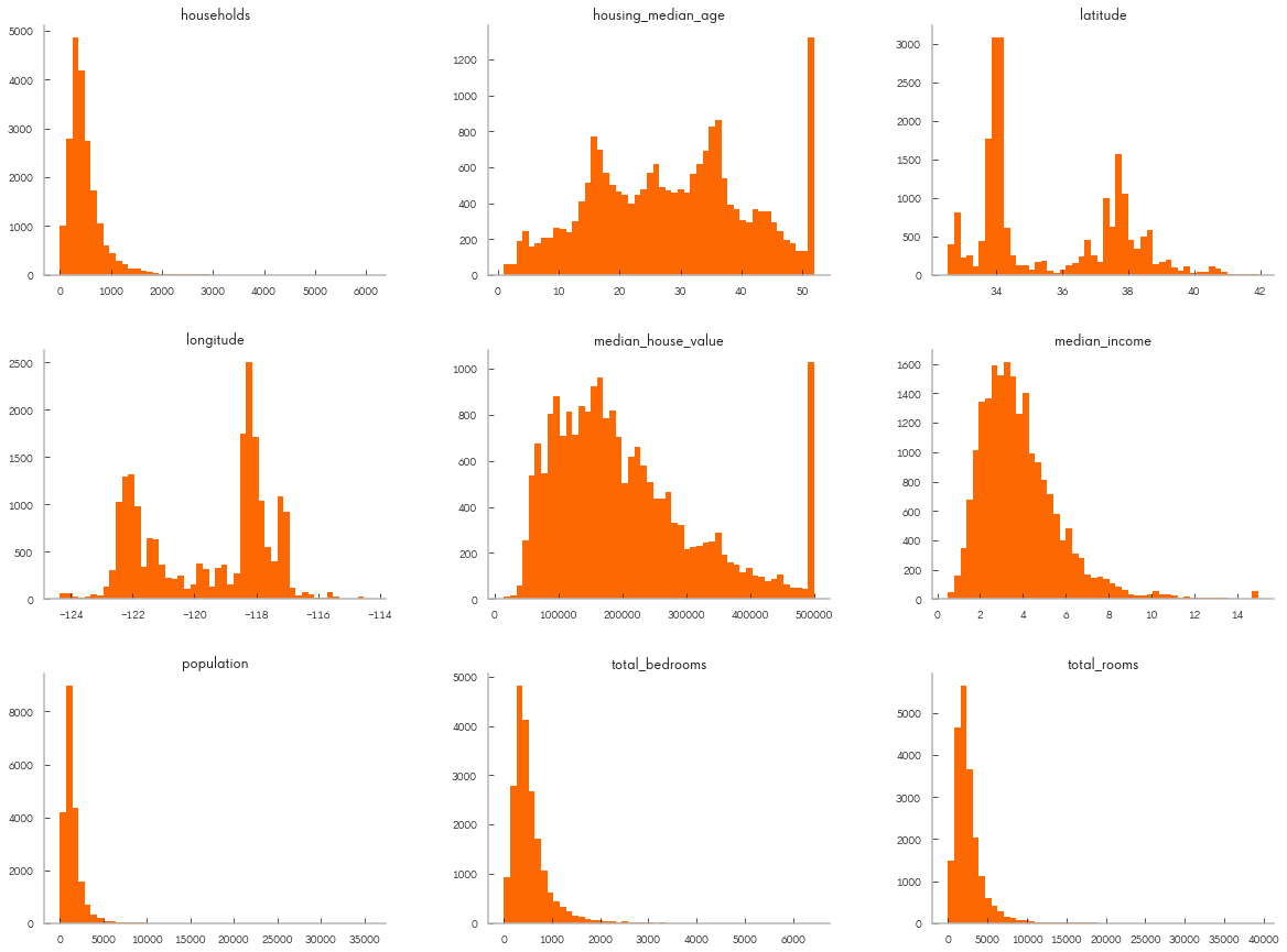
Split the data
Here we create training and test splits
[128]:
train_set, test_set = train_test_split(housing_df, test_size=0.2, random_state=8)
[129]:
train_set.head()
[129]:
| longitude | latitude | housing_median_age | total_rooms | total_bedrooms | population | households | median_income | median_house_value | ocean_proximity | |
|---|---|---|---|---|---|---|---|---|---|---|
| 17875 | -121.99 | 37.40 | 35.0 | 1845.0 | 325.0 | 1343.0 | 317.0 | 5.3912 | 235300.0 | <1H OCEAN |
| 9360 | -122.53 | 37.95 | 22.0 | 7446.0 | 1979.0 | 2980.0 | 1888.0 | 3.5838 | 271300.0 | NEAR BAY |
| 4338 | -118.31 | 34.08 | 26.0 | 1609.0 | 534.0 | 1868.0 | 497.0 | 2.7038 | 227100.0 | <1H OCEAN |
| 986 | -121.85 | 37.72 | 43.0 | 228.0 | 40.0 | 83.0 | 42.0 | 10.3203 | 400000.0 | INLAND |
| 8129 | -118.17 | 33.80 | 26.0 | 1589.0 | 380.0 | 883.0 | 366.0 | 3.5313 | 187500.0 | NEAR OCEAN |
[130]:
test_set.head()
[130]:
| longitude | latitude | housing_median_age | total_rooms | total_bedrooms | population | households | median_income | median_house_value | ocean_proximity | |
|---|---|---|---|---|---|---|---|---|---|---|
| 15722 | -122.46 | 37.78 | 47.0 | 1682.0 | 379.0 | 837.0 | 375.0 | 5.2806 | 400000.0 | NEAR BAY |
| 19685 | -121.61 | 39.14 | 44.0 | 2035.0 | 476.0 | 1030.0 | 453.0 | 1.4661 | 65200.0 | INLAND |
| 6989 | -118.04 | 33.97 | 29.0 | 2376.0 | 700.0 | 1968.0 | 680.0 | 2.6082 | 162500.0 | <1H OCEAN |
| 5804 | -118.25 | 34.15 | 13.0 | 1107.0 | 479.0 | 616.0 | 443.0 | 0.8185 | 187500.0 | <1H OCEAN |
| 5806 | -118.26 | 34.14 | 29.0 | 3431.0 | 1222.0 | 4094.0 | 1205.0 | 2.2614 | 248100.0 | <1H OCEAN |
reduce the number of categories
[172]:
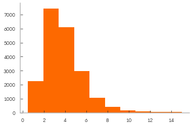
housing_df["median_income"].hist();
[173]:
# Create income category
# Divide by 1.5 to limit the number of income categories
housing_df["income_cat"] = np.ceil(housing_df["median_income"] / 1.5)
# Label those above 5 as 5
housing_df["income_cat"].where(housing_df["income_cat"] < 5, 5.0, inplace=True)
[174]:
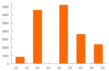
# plot histogram for new category
housing_df["income_cat"].hist();
[175]:
housing_df["income_cat"].value_counts()
[175]:
3.0    7236
2.0    6581
4.0    3639
5.0    2362
1.0     822
Name: income_cat, dtype: int64
From the above histogram we see the data is not evenly split. We stratify in order to properly represent population with splits.
Stratify data
[187]:
# split data again but this time with strata
split = StratifiedShuffleSplit(n_splits=1, test_size=0.2, random_state=42)
for train_index, test_index in split.split(housing_df, housing_df["income_cat"]):
    print('Size of training set: \t {}'.format(len(train_index)))
    print('Size of test set: \t {}'.format(len(test_index)))
    strat_train_set = housing_df.loc[train_index]
    strat_test_set = housing_df.loc[test_index]
Size of training set:    16512
Size of test set:        4128
[188]:
strat_test_set.shape
[188]:
(4128, 11)
[189]:
strat_train_set.shape
[189]:
(16512, 11)
[190]:
# strata ratios
strat_test_set["income_cat"].value_counts() / len(strat_test_set)
[190]:
3.0    0.350533
2.0    0.318798
4.0    0.176357
5.0    0.114583
1.0    0.039729
Name: income_cat, dtype: float64
[191]:
# compared to original population
housing_df["income_cat"].value_counts() / len(housing_df)
[191]:
3.0    0.350581
2.0    0.318847
4.0    0.176308
5.0    0.114438
1.0    0.039826
Name: income_cat, dtype: float64
[192]:
# Now we can drop the income cat column
for df in [strat_train_set, strat_test_set]:
    df.drop("income_cat", axis=1, inplace=True)
[193]:
strat_train_set.shape
[193]:
(16512, 10)
[194]:
strat_test_set.shape
[194]:
(4128, 10)
Save strata to pickles
[195]:
# Save the strata sets
strat_train_set.to_pickle('data/interim/'+'strat_train_set'+'.pkl')
strat_test_set.to_pickle('data/interim/'+'strat_test_set'+'.pkl')
[196]:
# read pickles to dataframes
strat_train_set = pd.read_pickle('data/interim/'+'strat_train_set'+'.pkl')
strat_test_set = pd.read_pickle('data/interim/'+'strat_test_set'+'.pkl')
Explore data (gain insights)
So far we have a general understanding of the data. Let’s go a little deeper. First we’ll make a copy of the data so we don’t alter the training set. Note: we are not working with the full data set from here on.
[199]:
housing_df = strat_train_set.copy()
[200]:
housing_df.shape
[200]:
(16512, 10)
[201]:
housing_df.plot(kind="scatter", x="longitude", y="latitude", alpha=0.1);
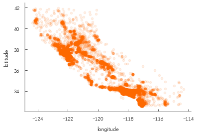
Looks like California!
[202]:
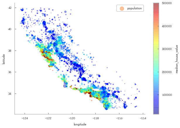
housing_df.plot(kind="scatter", x="longitude", y="latitude", alpha=0.4,
    s=housing_df["population"]/100, label="population", figsize=(10,7),
    c="median_house_value", cmap=plt.get_cmap("jet"), colorbar=True,
    sharex=False)
plt.legend();
[203]:
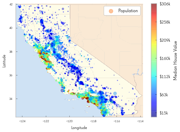
import matplotlib.image as mpimg
california_img=mpimg.imread( 'reports/figures/california.png')
ax = housing_df.plot(kind="scatter", x="longitude", y="latitude", figsize=(10,7),
                       s=housing_df['population']/100, label="Population",
                       c="median_house_value", cmap=plt.get_cmap("jet"),
                       colorbar=False, alpha=0.4,
                      )
plt.imshow(california_img, extent=[-124.55, -113.80, 32.45, 42.05], alpha=0.5,
           cmap=plt.get_cmap("jet"))
plt.ylabel("Latitude", fontsize=14)
plt.xlabel("Longitude", fontsize=14)

prices = housing_df["median_house_value"]
tick_values = np.linspace(prices.min(), prices.max(), 11)
cbar = plt.colorbar()
cbar.ax.set_yticklabels(["$%dk"%(round(v/1000)) for v in tick_values], fontsize=14)
cbar.set_label('Median House Value', fontsize=16)

plt.legend(fontsize=16)
plt.show()
[204]:
housing_df.corr()['median_house_value'].sort_values(ascending=False)
[204]:
median_house_value    1.000000
median_income         0.687160
total_rooms           0.135097
housing_median_age    0.114110
households            0.064506
total_bedrooms        0.047689
population           -0.026920
longitude            -0.047432
latitude             -0.142724
Name: median_house_value, dtype: float64
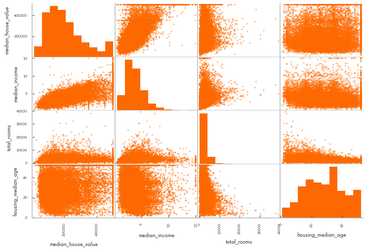
We see a strong correlation between median income and median house value. Next let’s look at the correlations.
[205]:
attributes = ["median_house_value", "median_income", "total_rooms",
              "housing_median_age"]
pd.plotting.scatter_matrix (housing_df[attributes], figsize=(12, 8));
[206]:
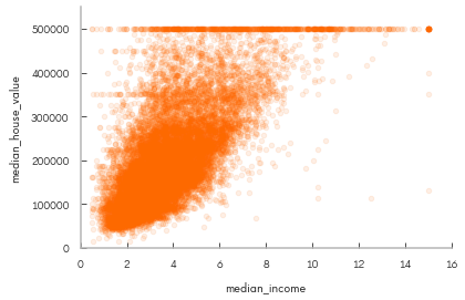
# Let's isolate median income and median house value
housing_df.plot(kind="scatter", x="median_income", y="median_house_value",
             alpha=0.1)
plt.axis([0, 16, 0, 550000])
[206]:
[0, 16, 0, 550000]
Experiment with Attribute Combinations
[207]:
housing_df["rooms_per_household"] = housing_df["total_rooms"]/housing_df["households"]
housing_df["bedrooms_per_room"] = housing_df["total_bedrooms"]/housing_df["total_rooms"]
housing_df["population_per_household"]=housing_df["population"]/housing_df["households"]
[208]:
# measure correlation again
housing_df.corr()['median_house_value'].sort_values(ascending=False)
[208]:
median_house_value          1.000000
median_income               0.687160
rooms_per_household         0.146285
total_rooms                 0.135097
housing_median_age          0.114110
households                  0.064506
total_bedrooms              0.047689
population_per_household   -0.021985
population                 -0.026920
longitude                  -0.047432
latitude                   -0.142724
bedrooms_per_room          -0.259984
Name: median_house_value, dtype: float64
[209]:
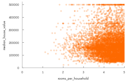
# We created two features (rooms_per_household and bedrooms_per_room) we mild correlation
housing_df.plot(kind="scatter", x="rooms_per_household", y="median_house_value",
             alpha=0.2)
plt.axis([0, 5, 0, 520000])
plt.show()
[210]:
# a bit of a sanity check, look at the new columns
housing_df.describe()
[210]:
| longitude | latitude | housing_median_age | total_rooms | total_bedrooms | population | households | median_income | median_house_value | rooms_per_household | bedrooms_per_room | population_per_household | |
|---|---|---|---|---|---|---|---|---|---|---|---|---|
| count | 16512.000000 | 16512.000000 | 16512.000000 | 16512.000000 | 16354.000000 | 16512.000000 | 16512.000000 | 16512.000000 | 16512.000000 | 16512.000000 | 16354.000000 | 16512.000000 |
| mean | -119.575834 | 35.639577 | 28.653101 | 2622.728319 | 534.973890 | 1419.790819 | 497.060380 | 3.875589 | 206990.920724 | 5.440341 | 0.212878 | 3.096437 |
| std | 2.001860 | 2.138058 | 12.574726 | 2138.458419 | 412.699041 | 1115.686241 | 375.720845 | 1.904950 | 115703.014830 | 2.611712 | 0.057379 | 11.584826 |
| min | -124.350000 | 32.540000 | 1.000000 | 6.000000 | 2.000000 | 3.000000 | 2.000000 | 0.499900 | 14999.000000 | 1.130435 | 0.100000 | 0.692308 |
| 25% | -121.800000 | 33.940000 | 18.000000 | 1443.000000 | 295.000000 | 784.000000 | 279.000000 | 2.566775 | 119800.000000 | 4.442040 | 0.175304 | 2.431287 |
| 50% | -118.510000 | 34.260000 | 29.000000 | 2119.500000 | 433.000000 | 1164.000000 | 408.000000 | 3.540900 | 179500.000000 | 5.232284 | 0.203031 | 2.817653 |
| 75% | -118.010000 | 37.720000 | 37.000000 | 3141.000000 | 644.000000 | 1719.250000 | 602.000000 | 4.744475 | 263900.000000 | 6.056361 | 0.239831 | 3.281420 |
| max | -114.310000 | 41.950000 | 52.000000 | 39320.000000 | 6210.000000 | 35682.000000 | 5358.000000 | 15.000100 | 500001.000000 | 141.909091 | 1.000000 | 1243.333333 |
We can always return to this step
Prepare data for Machine Learning algorithms
[211]:
# drop labels for training set
# here the drop method also creates a copy
housing = strat_train_set.drop("median_house_value", axis=1)
housing_labels = strat_train_set["median_house_value"].copy()
[212]:
housing.shape
[212]:
(16512, 9)
Explore missing data
[213]:
sample_incomplete_rows = housing[housing.isnull().any(axis=1)].head()
sample_incomplete_rows
[213]:
| longitude | latitude | housing_median_age | total_rooms | total_bedrooms | population | households | median_income | ocean_proximity | |
|---|---|---|---|---|---|---|---|---|---|
| 4629 | -118.30 | 34.07 | 18.0 | 3759.0 | NaN | 3296.0 | 1462.0 | 2.2708 | <1H OCEAN |
| 6068 | -117.86 | 34.01 | 16.0 | 4632.0 | NaN | 3038.0 | 727.0 | 5.1762 | <1H OCEAN |
| 17923 | -121.97 | 37.35 | 30.0 | 1955.0 | NaN | 999.0 | 386.0 | 4.6328 | <1H OCEAN |
| 13656 | -117.30 | 34.05 | 6.0 | 2155.0 | NaN | 1039.0 | 391.0 | 1.6675 | INLAND |
| 19252 | -122.79 | 38.48 | 7.0 | 6837.0 | NaN | 3468.0 | 1405.0 | 3.1662 | <1H OCEAN |
Three options to handle missing data
drop rows
[214]:
 # option 1
sample_incomplete_rows.dropna(subset=["total_bedrooms"])
[214]:
| longitude | latitude | housing_median_age | total_rooms | total_bedrooms | population | households | median_income | ocean_proximity |
|---|
drop attributes (columns)
[215]:
sample_incomplete_rows.drop("total_bedrooms", axis=1) # option 2
[215]:
| longitude | latitude | housing_median_age | total_rooms | population | households | median_income | ocean_proximity | |
|---|---|---|---|---|---|---|---|---|
| 4629 | -118.30 | 34.07 | 18.0 | 3759.0 | 3296.0 | 1462.0 | 2.2708 | <1H OCEAN |
| 6068 | -117.86 | 34.01 | 16.0 | 4632.0 | 3038.0 | 727.0 | 5.1762 | <1H OCEAN |
| 17923 | -121.97 | 37.35 | 30.0 | 1955.0 | 999.0 | 386.0 | 4.6328 | <1H OCEAN |
| 13656 | -117.30 | 34.05 | 6.0 | 2155.0 | 1039.0 | 391.0 | 1.6675 | INLAND |
| 19252 | -122.79 | 38.48 | 7.0 | 6837.0 | 3468.0 | 1405.0 | 3.1662 | <1H OCEAN |
impute data
[216]:
median = housing["total_bedrooms"].median()
sample_incomplete_rows["total_bedrooms"].fillna(median, inplace=True) # option 3
sample_incomplete_rows
[216]:
| longitude | latitude | housing_median_age | total_rooms | total_bedrooms | population | households | median_income | ocean_proximity | |
|---|---|---|---|---|---|---|---|---|---|
| 4629 | -118.30 | 34.07 | 18.0 | 3759.0 | 433.0 | 3296.0 | 1462.0 | 2.2708 | <1H OCEAN |
| 6068 | -117.86 | 34.01 | 16.0 | 4632.0 | 433.0 | 3038.0 | 727.0 | 5.1762 | <1H OCEAN |
| 17923 | -121.97 | 37.35 | 30.0 | 1955.0 | 433.0 | 999.0 | 386.0 | 4.6328 | <1H OCEAN |
| 13656 | -117.30 | 34.05 | 6.0 | 2155.0 | 433.0 | 1039.0 | 391.0 | 1.6675 | INLAND |
| 19252 | -122.79 | 38.48 | 7.0 | 6837.0 | 433.0 | 3468.0 | 1405.0 | 3.1662 | <1H OCEAN |
[217]:
# Use the sklearn imputer class, select median as method
from sklearn.impute import SimpleImputer
imputer = SimpleImputer(strategy="median")
[218]:
# remove text data, cannot impute
# create copy
housing_num = housing.drop('ocean_proximity', axis=1)

# run imputer on numerical data
imputer.fit(housing_num)
[218]:
SimpleImputer(copy=True, fill_value=None, missing_values=nan,
       strategy='median', verbose=0)
[219]:
# peak into estimators
imputer.statistics_
[219]:
array([-118.51  ,   34.26  ,   29.    , 2119.5   ,  433.    , 1164.    ,
        408.    ,    3.5409])
[220]:
# sanity check values
housing_num.median().values
[220]:
array([-118.51  ,   34.26  ,   29.    , 2119.5   ,  433.    , 1164.    ,
        408.    ,    3.5409])
Tranfsform training set
[221]:
X = imputer.transform(housing_num)
[222]:
# convert back into dataframe
housing_tr = pd.DataFrame(X, columns=housing_num.columns,
                          index = housing.index.values)
housing_tr.head()
[222]:
| longitude | latitude | housing_median_age | total_rooms | total_bedrooms | population | households | median_income | |
|---|---|---|---|---|---|---|---|---|
| 17606 | -121.89 | 37.29 | 38.0 | 1568.0 | 351.0 | 710.0 | 339.0 | 2.7042 |
| 18632 | -121.93 | 37.05 | 14.0 | 679.0 | 108.0 | 306.0 | 113.0 | 6.4214 |
| 14650 | -117.20 | 32.77 | 31.0 | 1952.0 | 471.0 | 936.0 | 462.0 | 2.8621 |
| 3230 | -119.61 | 36.31 | 25.0 | 1847.0 | 371.0 | 1460.0 | 353.0 | 1.8839 |
| 3555 | -118.59 | 34.23 | 17.0 | 6592.0 | 1525.0 | 4459.0 | 1463.0 | 3.0347 |
[223]:
# look at imputed data
housing_tr.loc[sample_incomplete_rows.index.values]
[223]:
| longitude | latitude | housing_median_age | total_rooms | total_bedrooms | population | households | median_income | |
|---|---|---|---|---|---|---|---|---|
| 4629 | -118.30 | 34.07 | 18.0 | 3759.0 | 433.0 | 3296.0 | 1462.0 | 2.2708 |
| 6068 | -117.86 | 34.01 | 16.0 | 4632.0 | 433.0 | 3038.0 | 727.0 | 5.1762 |
| 17923 | -121.97 | 37.35 | 30.0 | 1955.0 | 433.0 | 999.0 | 386.0 | 4.6328 |
| 13656 | -117.30 | 34.05 | 6.0 | 2155.0 | 433.0 | 1039.0 | 391.0 | 1.6675 |
| 19252 | -122.79 | 38.48 | 7.0 | 6837.0 | 433.0 | 3468.0 | 1405.0 | 3.1662 |
[224]:
# clean index this time
housing_tr = pd.DataFrame(X, columns=housing_num.columns)
housing_tr.head()
[224]:
| longitude | latitude | housing_median_age | total_rooms | total_bedrooms | population | households | median_income | |
|---|---|---|---|---|---|---|---|---|
| 0 | -121.89 | 37.29 | 38.0 | 1568.0 | 351.0 | 710.0 | 339.0 | 2.7042 |
| 1 | -121.93 | 37.05 | 14.0 | 679.0 | 108.0 | 306.0 | 113.0 | 6.4214 |
| 2 | -117.20 | 32.77 | 31.0 | 1952.0 | 471.0 | 936.0 | 462.0 | 2.8621 |
| 3 | -119.61 | 36.31 | 25.0 | 1847.0 | 371.0 | 1460.0 | 353.0 | 1.8839 |
| 4 | -118.59 | 34.23 | 17.0 | 6592.0 | 1525.0 | 4459.0 | 1463.0 | 3.0347 |
Text Encoding
[225]:
from sklearn.preprocessing import OneHotEncoder
[226]:
housing_cat = housing[['ocean_proximity']]
housing_cat.head()
[226]:
| ocean_proximity | |
|---|---|
| 17606 | <1H OCEAN |
| 18632 | <1H OCEAN |
| 14650 | NEAR OCEAN |
| 3230 | INLAND |
| 3555 | <1H OCEAN |
[227]:
cat_encoder =  OneHotEncoder()
housing_cat_1hot = cat_encoder.fit_transform(housing_cat)
housing_cat_1hot
[227]:
<16512x5 sparse matrix of type '<class 'numpy.float64'>'
    with 16512 stored elements in Compressed Sparse Row format>
[228]:
# to see full array
housing_cat_1hot.toarray()
[228]:
array([[1., 0., 0., 0., 0.],
       [1., 0., 0., 0., 0.],
       [0., 0., 0., 0., 1.],
       ...,
       [0., 1., 0., 0., 0.],
       [1., 0., 0., 0., 0.],
       [0., 0., 0., 1., 0.]])
[229]:
# view categories text
cat_encoder.categories_
[229]:
[array(['<1H OCEAN', 'INLAND', 'ISLAND', 'NEAR BAY', 'NEAR OCEAN'],
       dtype=object)]
Custom Transformers
[230]:
list(housing.columns).index("total_rooms")
[230]:
3
[231]:
from sklearn.base import BaseEstimator, TransformerMixin

# get the right column indices: safer than hard-coding indices 3, 4, 5, 6
rooms_ix, bedrooms_ix, population_ix, household_ix = [
    list(housing.columns).index(col)
    for col in ("total_rooms", "total_bedrooms", "population", "households")]

class CombinedAttributesAdder(BaseEstimator, TransformerMixin):
    def __init__(self, add_bedrooms_per_room = True): # no *args or **kargs
        self.add_bedrooms_per_room = add_bedrooms_per_room
    def fit(self, X, y=None):
        return self  # nothing else to do
    def transform(self, X, y=None):
        rooms_per_household = X[:, rooms_ix] / X[:, household_ix]
        population_per_household = X[:, population_ix] / X[:, household_ix]
        if self.add_bedrooms_per_room:
            bedrooms_per_room = X[:, bedrooms_ix] / X[:, rooms_ix]
            return np.c_[X, rooms_per_household, population_per_household,
                         bedrooms_per_room]
        else:
            return np.c_[X, rooms_per_household, population_per_household]

attr_adder = CombinedAttributesAdder(add_bedrooms_per_room=False)
housing_extra_attribs = attr_adder.transform(housing.values)
[232]:
# Yet another method
from sklearn.preprocessing import FunctionTransformer

def add_extra_features(X, add_bedrooms_per_room=True):
    rooms_per_household = X[:, rooms_ix] / X[:, household_ix]
    population_per_household = X[:, population_ix] / X[:, household_ix]
    if add_bedrooms_per_room:
        bedrooms_per_room = X[:, bedrooms_ix] / X[:, rooms_ix]
        return np.c_[X, rooms_per_household, population_per_household,
                     bedrooms_per_room]
    else:
        return np.c_[X, rooms_per_household, population_per_household]

attr_adder = FunctionTransformer(add_extra_features, validate=False,
                                 kw_args={"add_bedrooms_per_room": False})
housing_extra_attribs = attr_adder.fit_transform(housing.values)
[233]:
housing_extra_attribs[0:3]
[233]:
array([[-121.89, 37.29, 38.0, 1568.0, 351.0, 710.0, 339.0, 2.7042,
        '<1H OCEAN', 4.625368731563422, 2.094395280235988],
       [-121.93, 37.05, 14.0, 679.0, 108.0, 306.0, 113.0, 6.4214,
        '<1H OCEAN', 6.008849557522124, 2.7079646017699117],
       [-117.2, 32.77, 31.0, 1952.0, 471.0, 936.0, 462.0, 2.8621,
        'NEAR OCEAN', 4.225108225108225, 2.0259740259740258]],
      dtype=object)
[234]:
housing_extra_attribs = pd.DataFrame(housing_extra_attribs, columns=list(
    housing.columns)+["rooms_per_household", "population_per_household"])
housing_extra_attribs.head()
[234]:
| longitude | latitude | housing_median_age | total_rooms | total_bedrooms | population | households | median_income | ocean_proximity | rooms_per_household | population_per_household | |
|---|---|---|---|---|---|---|---|---|---|---|---|
| 0 | -121.89 | 37.29 | 38 | 1568 | 351 | 710 | 339 | 2.7042 | <1H OCEAN | 4.62537 | 2.0944 |
| 1 | -121.93 | 37.05 | 14 | 679 | 108 | 306 | 113 | 6.4214 | <1H OCEAN | 6.00885 | 2.70796 |
| 2 | -117.2 | 32.77 | 31 | 1952 | 471 | 936 | 462 | 2.8621 | NEAR OCEAN | 4.22511 | 2.02597 |
| 3 | -119.61 | 36.31 | 25 | 1847 | 371 | 1460 | 353 | 1.8839 | INLAND | 5.23229 | 4.13598 |
| 4 | -118.59 | 34.23 | 17 | 6592 | 1525 | 4459 | 1463 | 3.0347 | <1H OCEAN | 4.50581 | 3.04785 |
Transformation Pipelines
[235]:
from sklearn.pipeline import Pipeline
from sklearn.preprocessing import StandardScaler

num_pipeline = Pipeline([
        ('imputer', SimpleImputer(strategy="median")),
        ('attribs_adder', FunctionTransformer(add_extra_features, validate=False)),
        ('std_scaler', StandardScaler()),
    ])

housing_num_tr = num_pipeline.fit_transform(housing_num)
[236]:
housing_num_tr.shape
[236]:
(16512, 11)
[237]:
housing_num_tr
[237]:
array([[-1.15604281,  0.77194962,  0.74333089, ..., -0.31205452,
        -0.08649871,  0.15531753],
       [-1.17602483,  0.6596948 , -1.1653172 , ...,  0.21768338,
        -0.03353391, -0.83628902],
       [ 1.18684903, -1.34218285,  0.18664186, ..., -0.46531516,
        -0.09240499,  0.4222004 ],
       ...,
       [ 1.58648943, -0.72478134, -1.56295222, ...,  0.3469342 ,
        -0.03055414, -0.52177644],
       [ 0.78221312, -0.85106801,  0.18664186, ...,  0.02499488,
         0.06150916, -0.30340741],
       [-1.43579109,  0.99645926,  1.85670895, ..., -0.22852947,
        -0.09586294,  0.10180567]])
[238]:
# Now we can combine both pipelines numerical and categorical into one
from sklearn.compose import ColumnTransformer
num_attribs = list(housing_num)
cat_attribs = ["ocean_proximity"]

full_pipeline = ColumnTransformer([
        ("num", num_pipeline, num_attribs),
        ("cat", OneHotEncoder(), cat_attribs),
    ])

housing_prepared = full_pipeline.fit_transform(housing)
[239]:
housing_prepared
[239]:
array([[-1.15604281,  0.77194962,  0.74333089, ...,  0.        ,
         0.        ,  0.        ],
       [-1.17602483,  0.6596948 , -1.1653172 , ...,  0.        ,
         0.        ,  0.        ],
       [ 1.18684903, -1.34218285,  0.18664186, ...,  0.        ,
         0.        ,  1.        ],
       ...,
       [ 1.58648943, -0.72478134, -1.56295222, ...,  0.        ,
         0.        ,  0.        ],
       [ 0.78221312, -0.85106801,  0.18664186, ...,  0.        ,
         0.        ,  0.        ],
       [-1.43579109,  0.99645926,  1.85670895, ...,  0.        ,
         1.        ,  0.        ]])
[240]:
housing_prepared.shape
[240]:
(16512, 16)
The new matrix contains the original columns transformed plus 5 more columns for the categorical encoder data
[241]:
# Save the transformed data
from sklearn.externals import joblib
joblib.dump(housing_prepared, 'data/interim/'+'housing_prepared'+'.pkl')
joblib.dump(housing_labels, 'data/interim/'+'housing_labels'+'.pkl')
[241]:
['data/interim/housing_labels.pkl']
Explore models
[242]:
# Load saved transformed data
from sklearn.externals import joblib
housing_prepared = joblib.load('data/interim/'+'housing_prepared'+'.pkl')
housing_labels = joblib.load('data/interim/'+'housing_labels'+'.pkl')
[244]:
housing_prepared.shape
[244]:
(16512, 16)
Linear Regression
[245]:
from sklearn.linear_model import LinearRegression

# instantiate model
lin_reg = LinearRegression()
# feed the model data and labels
lin_reg.fit(housing_prepared, housing_labels)
[245]:
LinearRegression(copy_X=True, fit_intercept=True, n_jobs=None,
         normalize=False)
[246]:
# let's try the full preprocessing pipeline on a few training instances
some_data = housing_df.iloc[:5]
some_labels = housing_labels.iloc[:5]
some_data_prepared = full_pipeline.transform(some_data)

print("Predictions:", lin_reg.predict(some_data_prepared))
Predictions: [210644.60459286 317768.80697211 210956.43331178  59218.98886849
 189747.55849879]
[247]:
print("Labels:", list(some_labels))
Labels: [286600.0, 340600.0, 196900.0, 46300.0, 254500.0]
[248]:
for pred, label in zip( lin_reg.predict(some_data_prepared), list(some_labels) ):
    print('Prediction: {} \t Label: {} '.format(int(pred),int( label)))
Prediction: 210644       Label: 286600
Prediction: 317768       Label: 340600
Prediction: 210956       Label: 196900
Prediction: 59218        Label: 46300
Prediction: 189747       Label: 254500
[249]:
pd.DataFrame({'Predictions': list( lin_reg.predict(some_data_prepared)) , 'Labels': list(some_labels)})
[249]:
| Labels | Predictions | |
|---|---|---|
| 0 | 286600.0 | 210644.604593 |
| 1 | 340600.0 | 317768.806972 |
| 2 | 196900.0 | 210956.433312 |
| 3 | 46300.0 | 59218.988868 |
| 4 | 254500.0 | 189747.558499 |
Model performance
[250]:
from sklearn.metrics import mean_squared_error

housing_predictions = lin_reg.predict(housing_prepared)
lin_mse = mean_squared_error(housing_labels, housing_predictions)
lin_rmse = np.sqrt(lin_mse)
lin_rmse
[250]:
68628.19819848922
[251]:
from sklearn.metrics import mean_absolute_error

lin_mae = mean_absolute_error(housing_labels, housing_predictions)
lin_mae
[251]:
49439.89599001898
Decision Tree
[252]:
from sklearn.tree import DecisionTreeRegressor

tree_reg = DecisionTreeRegressor(random_state=42)
tree_reg.fit(housing_prepared, housing_labels)
[252]:
DecisionTreeRegressor(criterion='mse', max_depth=None, max_features=None,
           max_leaf_nodes=None, min_impurity_decrease=0.0,
           min_impurity_split=None, min_samples_leaf=1,
           min_samples_split=2, min_weight_fraction_leaf=0.0,
           presort=False, random_state=42, splitter='best')
[253]:
housing_predictions = tree_reg.predict(housing_prepared)
tree_mse = mean_squared_error(housing_labels, housing_predictions)
tree_rmse = np.sqrt(tree_mse)
tree_rmse
[253]:
0.0
Model Performance
[254]:
pd.DataFrame({'Predictions': list(housing_predictions) , 'Labels': list(housing_labels)}).head()
[254]:
| Labels | Predictions | |
|---|---|---|
| 0 | 286600.0 | 286600.0 |
| 1 | 340600.0 | 340600.0 |
| 2 | 196900.0 | 196900.0 |
| 3 | 46300.0 | 46300.0 |
| 4 | 254500.0 | 254500.0 |
Fine tune model
Decision Tree Regression
[255]:
from sklearn.model_selection import cross_val_score

scores = cross_val_score(tree_reg, housing_prepared, housing_labels,
                         scoring="neg_mean_squared_error", cv=10)
# cv expects a utility function instead of cost function
tree_rmse_scores = np.sqrt(-scores)
[256]:
def display_scores(scores):
    print("Scores:", scores)
    print("Mean:", scores.mean())
    print("Standard deviation:", scores.std())

display_scores(tree_rmse_scores)
Scores: [70194.33680785 66855.16363941 72432.58244769 70758.73896782
 71115.88230639 75585.14172901 70262.86139133 70273.6325285
 75366.87952553 71231.65726027]
Mean: 71407.68766037929
Standard deviation: 2439.4345041191004
This is peforming worse than linear regression
Linear Regression
[257]:
lin_scores = cross_val_score(lin_reg, housing_prepared, housing_labels,
                             scoring="neg_mean_squared_error", cv=10)
lin_rmse_scores = np.sqrt(-lin_scores)
display_scores(lin_rmse_scores)
Scores: [66782.73843989 66960.118071   70347.95244419 74739.57052552
 68031.13388938 71193.84183426 64969.63056405 68281.61137997
 71552.91566558 67665.10082067]
Mean: 69052.46136345083
Standard deviation: 2731.674001798347
Random Forrest Regression
[258]:
from sklearn.ensemble import RandomForestRegressor

forest_reg = RandomForestRegressor(n_estimators=10, random_state=42)
forest_reg.fit(housing_prepared, housing_labels)
[258]:
RandomForestRegressor(bootstrap=True, criterion='mse', max_depth=None,
           max_features='auto', max_leaf_nodes=None,
           min_impurity_decrease=0.0, min_impurity_split=None,
           min_samples_leaf=1, min_samples_split=2,
           min_weight_fraction_leaf=0.0, n_estimators=10, n_jobs=None,
           oob_score=False, random_state=42, verbose=0, warm_start=False)
[259]:
housing_predictions = forest_reg.predict(housing_prepared)
forest_mse = mean_squared_error(housing_labels, housing_predictions)
forest_rmse = np.sqrt(forest_mse)
forest_rmse
[259]:
21933.31414779769
[260]:
from sklearn.model_selection import cross_val_score

forest_scores = cross_val_score(forest_reg, housing_prepared, housing_labels,
                                scoring="neg_mean_squared_error", cv=10)
forest_rmse_scores = np.sqrt(-forest_scores)
display_scores(forest_rmse_scores)
Scores: [51646.44545909 48940.60114882 53050.86323649 54408.98730149
 50922.14870785 56482.50703987 51864.52025526 49760.85037653
 55434.21627933 53326.10093303]
Mean: 52583.72407377466
Standard deviation: 2298.353351147122
Support Vector Machines (linear kernel)
A low C makes the decision surface smooth, while a high C aims at classifying all training examples correctly. gamma defines how much influence a single training example has. The larger gamma is, the closer other examples must be to be affected.
[261]:
from sklearn.svm import SVR

svm_reg = SVR(kernel="linear")
svm_reg.fit(housing_prepared, housing_labels)
housing_predictions = svm_reg.predict(housing_prepared)
svm_mse = mean_squared_error(housing_labels, housing_predictions)
svm_rmse = np.sqrt(svm_mse)
svm_rmse
[261]:
111094.6308539982
[262]:
svm_scores = cross_val_score(svm_reg, housing_prepared, housing_labels,
                             scoring="neg_mean_squared_error", cv=10)
svm_rmse_scores = np.sqrt(-svm_scores)
display_scores(svm_rmse_scores)
Scores: [105342.09141998 112489.24624123 110092.35042753 113403.22892482
 110638.90119657 115675.8320024  110703.56887243 114476.89008206
 113756.17971227 111520.1120808 ]
Mean: 111809.84009600841
Standard deviation: 2762.393664321567
[263]:
# rbf kernel
svm_reg = SVR(kernel="rbf", gamma='auto')
svm_reg.fit(housing_prepared, housing_labels)
housing_predictions = svm_reg.predict(housing_prepared)
svm_mse = mean_squared_error(housing_labels, housing_predictions)
svm_rmse = np.sqrt(svm_mse)
svm_rmse
[263]:
118577.43356412371
[264]:
svm_scores = cross_val_score(svm_reg, housing_prepared, housing_labels,
                             scoring="neg_mean_squared_error", cv=10)
svm_rmse_scores = np.sqrt(-svm_scores)
display_scores(svm_rmse_scores)
Scores: [111393.33263237 119546.71049753 116961.00489445 120449.0155974
 117622.20149716 122303.76986818 117640.09907103 121459.63518806
 120348.51364519 118025.61954959]
Mean: 118574.99024409598
Standard deviation: 2934.1329433145675
Grid Search
- Grid search helps you find the best hyper parameters
- In the case below there will be \((3*4 + 2*3)*5=(12 + 6)*5 = 90\) trainings
[265]:
from sklearn.model_selection import GridSearchCV

param_grid = [
    # try 12 (3×4) combinations of hyperparameters
    {'n_estimators': [3, 10, 30], 'max_features': [2, 4, 6, 8]},
    # then try 6 (2×3) combinations with bootstrap set as False
    {'bootstrap': [False], 'n_estimators': [3, 10], 'max_features': [2, 3, 4]},
  ]

forest_reg = RandomForestRegressor(random_state=42)
# train across 5 folds, that's a total of (12+6)*5=90 rounds of training
grid_search = GridSearchCV(forest_reg, param_grid, cv=5,n_jobs=-1,
                           scoring='neg_mean_squared_error', return_train_score=True)
grid_search.fit(housing_prepared, housing_labels)
[265]:
GridSearchCV(cv=5, error_score='raise-deprecating',
       estimator=RandomForestRegressor(bootstrap=True, criterion='mse', max_depth=None,
           max_features='auto', max_leaf_nodes=None,
           min_impurity_decrease=0.0, min_impurity_split=None,
           min_samples_leaf=1, min_samples_split=2,
           min_weight_fraction_leaf=0.0, n_estimators='warn', n_jobs=None,
           oob_score=False, random_state=42, verbose=0, warm_start=False),
       fit_params=None, iid='warn', n_jobs=-1,
       param_grid=[{'n_estimators': [3, 10, 30], 'max_features': [2, 4, 6, 8]}, {'n_estimators': [3, 10], 'max_features': [2, 3, 4], 'bootstrap': [False]}],
       pre_dispatch='2*n_jobs', refit=True, return_train_score=True,
       scoring='neg_mean_squared_error', verbose=0)
[266]:
print('The best hyperparameter combination found: {}'.format(grid_search.best_params_))
The best hyperparameter combination found: {'n_estimators': 30, 'max_features': 8}
[267]:
# parameters for best estimator
grid_search.best_estimator_
[267]:
RandomForestRegressor(bootstrap=True, criterion='mse', max_depth=None,
           max_features=8, max_leaf_nodes=None, min_impurity_decrease=0.0,
           min_impurity_split=None, min_samples_leaf=1,
           min_samples_split=2, min_weight_fraction_leaf=0.0,
           n_estimators=30, n_jobs=None, oob_score=False, random_state=42,
           verbose=0, warm_start=False)
Looking at the score for each hyper parameters combination
[268]:
cvres = grid_search.cv_results_
for mean_score, params in zip(cvres["mean_test_score"], cvres["params"]):
    print(int(np.sqrt(-mean_score)), params)
63669 {'n_estimators': 3, 'max_features': 2}
55627 {'n_estimators': 10, 'max_features': 2}
53384 {'n_estimators': 30, 'max_features': 2}
60965 {'n_estimators': 3, 'max_features': 4}
52740 {'n_estimators': 10, 'max_features': 4}
50377 {'n_estimators': 30, 'max_features': 4}
58663 {'n_estimators': 3, 'max_features': 6}
52006 {'n_estimators': 10, 'max_features': 6}
50146 {'n_estimators': 30, 'max_features': 6}
57869 {'n_estimators': 3, 'max_features': 8}
51711 {'n_estimators': 10, 'max_features': 8}
49682 {'n_estimators': 30, 'max_features': 8}
62895 {'n_estimators': 3, 'max_features': 2, 'bootstrap': False}
54658 {'n_estimators': 10, 'max_features': 2, 'bootstrap': False}
59470 {'n_estimators': 3, 'max_features': 3, 'bootstrap': False}
52725 {'n_estimators': 10, 'max_features': 3, 'bootstrap': False}
57490 {'n_estimators': 3, 'max_features': 4, 'bootstrap': False}
51009 {'n_estimators': 10, 'max_features': 4, 'bootstrap': False}
[269]:
pd.DataFrame(grid_search.cv_results_).sort_values(by='rank_test_score')
[269]:
| mean_fit_time | mean_score_time | mean_test_score | mean_train_score | param_bootstrap | param_max_features | param_n_estimators | params | rank_test_score | split0_test_score | ... | split2_test_score | split2_train_score | split3_test_score | split3_train_score | split4_test_score | split4_train_score | std_fit_time | std_score_time | std_test_score | std_train_score | |
|---|---|---|---|---|---|---|---|---|---|---|---|---|---|---|---|---|---|---|---|---|---|
| 11 | 3.354504 | 0.053489 | -2.468326e+09 | -3.810330e+08 | NaN | 8 | 30 | {'n_estimators': 30, 'max_features': 8} | 1 | -2.357390e+09 | ... | -2.591972e+09 | -3.773239e+08 | -2.318617e+09 | -3.882250e+08 | -2.527022e+09 | -3.810005e+08 | 0.172000 | 0.009551 | 1.091647e+08 | 4.871017e+06 |
| 8 | 2.525017 | 0.050918 | -2.514668e+09 | -3.841296e+08 | NaN | 6 | 30 | {'n_estimators': 30, 'max_features': 6} | 2 | -2.370010e+09 | ... | -2.607703e+09 | -3.805218e+08 | -2.350953e+09 | -3.856095e+08 | -2.661059e+09 | -3.901917e+08 | 0.221924 | 0.002579 | 1.285063e+08 | 3.617057e+06 |
| 5 | 1.784167 | 0.058159 | -2.537877e+09 | -3.879289e+08 | NaN | 4 | 30 | {'n_estimators': 30, 'max_features': 4} | 3 | -2.387153e+09 | ... | -2.666426e+09 | -3.790867e+08 | -2.398071e+09 | -4.040957e+08 | -2.649316e+09 | -3.845520e+08 | 0.122772 | 0.017129 | 1.214603e+08 | 8.571233e+06 |
| 17 | 0.976491 | 0.028234 | -2.601971e+09 | -3.028238e-03 | False | 4 | 10 | {'n_estimators': 10, 'max_features': 4, 'boots... | 4 | -2.525578e+09 | ... | -2.609100e+09 | -0.000000e+00 | -2.439607e+09 | -0.000000e+00 | -2.725548e+09 | -0.000000e+00 | 0.295675 | 0.007139 | 1.088031e+08 | 6.056477e-03 |
| 10 | 1.112599 | 0.019048 | -2.674037e+09 | -4.923911e+08 | NaN | 8 | 10 | {'n_estimators': 10, 'max_features': 8} | 5 | -2.571970e+09 | ... | -2.842317e+09 | -4.730979e+08 | -2.460258e+09 | -5.155367e+08 | -2.776666e+09 | -4.985555e+08 | 0.100974 | 0.002301 | 1.392720e+08 | 1.459294e+07 |
| 7 | 0.827751 | 0.020989 | -2.704640e+09 | -5.013349e+08 | NaN | 6 | 10 | {'n_estimators': 10, 'max_features': 6} | 6 | -2.549663e+09 | ... | -2.762720e+09 | -4.994664e+08 | -2.521134e+09 | -4.990325e+08 | -2.907667e+09 | -5.055542e+08 | 0.077836 | 0.006335 | 1.471542e+08 | 3.100456e+06 |
| 15 | 0.675495 | 0.022814 | -2.779927e+09 | -5.272080e+00 | False | 3 | 10 | {'n_estimators': 10, 'max_features': 3, 'boots... | 7 | -2.757999e+09 | ... | -2.830927e+09 | -0.000000e+00 | -2.672765e+09 | -0.000000e+00 | -2.786190e+09 | -5.465556e+00 | 0.073931 | 0.001319 | 6.286611e+07 | 8.093117e+00 |
| 4 | 0.558351 | 0.021956 | -2.781611e+09 | -5.163863e+08 | NaN | 4 | 10 | {'n_estimators': 10, 'max_features': 4} | 8 | -2.666283e+09 | ... | -2.892276e+09 | -4.962893e+08 | -2.616813e+09 | -5.436192e+08 | -2.948207e+09 | -5.160297e+08 | 0.039796 | 0.008723 | 1.268562e+08 | 1.542862e+07 |
| 2 | 1.151661 | 0.052023 | -2.849913e+09 | -4.394734e+08 | NaN | 2 | 30 | {'n_estimators': 30, 'max_features': 2} | 9 | -2.689185e+09 | ... | -2.948330e+09 | -4.371702e+08 | -2.619995e+09 | -4.376955e+08 | -2.970968e+09 | -4.452654e+08 | 0.144397 | 0.002657 | 1.626879e+08 | 2.966320e+06 |
| 13 | 0.611461 | 0.023005 | -2.987513e+09 | -6.056027e-01 | False | 2 | 10 | {'n_estimators': 10, 'max_features': 2, 'boots... | 10 | -2.810721e+09 | ... | -3.131187e+09 | -0.000000e+00 | -2.788537e+09 | -0.000000e+00 | -3.099347e+09 | -2.967449e+00 | 0.043821 | 0.000978 | 1.539231e+08 | 1.181156e+00 |
| 1 | 0.373621 | 0.023403 | -3.094381e+09 | -5.818785e+08 | NaN | 2 | 10 | {'n_estimators': 10, 'max_features': 2} | 11 | -3.047771e+09 | ... | -3.130196e+09 | -5.776964e+08 | -2.865188e+09 | -5.716332e+08 | -3.173856e+09 | -5.802501e+08 | 0.079333 | 0.005578 | 1.327046e+08 | 7.345821e+06 |
| 16 | 0.253212 | 0.007124 | -3.305171e+09 | 0.000000e+00 | False | 4 | 3 | {'n_estimators': 3, 'max_features': 4, 'bootst... | 12 | -3.134040e+09 | ... | -3.440422e+09 | -0.000000e+00 | -3.053647e+09 | -0.000000e+00 | -3.338344e+09 | -0.000000e+00 | 0.097383 | 0.000550 | 1.879203e+08 | 0.000000e+00 |
| 9 | 0.280610 | 0.006559 | -3.348851e+09 | -8.883545e+08 | NaN | 8 | 3 | {'n_estimators': 3, 'max_features': 8} | 13 | -3.353504e+09 | ... | -3.402843e+09 | -8.603321e+08 | -3.129307e+09 | -8.881964e+08 | -3.510047e+09 | -9.151287e+08 | 0.043096 | 0.000172 | 1.241864e+08 | 2.750227e+07 |
| 6 | 0.129712 | 0.006625 | -3.441447e+09 | -9.023976e+08 | NaN | 6 | 3 | {'n_estimators': 3, 'max_features': 6} | 14 | -3.119657e+09 | ... | -3.592772e+09 | -9.353135e+08 | -3.328934e+09 | -9.009801e+08 | -3.579607e+09 | -8.624664e+08 | 0.020992 | 0.000224 | 1.893141e+08 | 2.591445e+07 |
| 14 | 0.216452 | 0.007962 | -3.536728e+09 | -1.214568e+01 | False | 3 | 3 | {'n_estimators': 3, 'max_features': 3, 'bootst... | 15 | -3.618324e+09 | ... | -3.554815e+09 | -0.000000e+00 | -3.619116e+09 | -0.000000e+00 | -3.449864e+09 | -6.072840e+01 | 0.081226 | 0.000395 | 7.795196e+07 | 2.429136e+01 |
| 3 | 0.143291 | 0.007133 | -3.716852e+09 | -9.848396e+08 | NaN | 4 | 3 | {'n_estimators': 3, 'max_features': 4} | 16 | -3.730181e+09 | ... | -3.734515e+09 | -9.169425e+08 | -3.418747e+09 | -1.037400e+09 | -3.913907e+09 | -9.707739e+08 | 0.027455 | 0.001225 | 1.631421e+08 | 4.084607e+07 |
| 12 | 0.137781 | 0.007999 | -3.955792e+09 | 0.000000e+00 | False | 2 | 3 | {'n_estimators': 3, 'max_features': 2, 'bootst... | 17 | -3.785816e+09 | ... | -4.061751e+09 | -0.000000e+00 | -3.675704e+09 | -0.000000e+00 | -4.089667e+09 | -0.000000e+00 | 0.022286 | 0.000159 | 1.900966e+08 | 0.000000e+00 |
| 0 | 0.177232 | 0.007945 | -4.053749e+09 | -1.105559e+09 | NaN | 2 | 3 | {'n_estimators': 3, 'max_features': 2} | 18 | -3.837622e+09 | ... | -4.196408e+09 | -1.116550e+09 | -3.903319e+09 | -1.112342e+09 | -4.184325e+09 | -1.129650e+09 | 0.034350 | 0.001114 | 1.519609e+08 | 2.220402e+07 |
18 rows × 23 columns
Randomized Search
[270]:
from sklearn.model_selection import RandomizedSearchCV
from scipy.stats import randint

param_distribs = {
        'n_estimators': randint(low=1, high=200),
        'max_features': randint(low=1, high=8),
    }

forest_reg = RandomForestRegressor(random_state=42)
rnd_search = RandomizedSearchCV(forest_reg, param_distributions=param_distribs, n_jobs=-1,
                                n_iter=10, cv=5, scoring='neg_mean_squared_error', random_state=42)
rnd_search.fit(housing_prepared, housing_labels)
[270]:
RandomizedSearchCV(cv=5, error_score='raise-deprecating',
          estimator=RandomForestRegressor(bootstrap=True, criterion='mse', max_depth=None,
           max_features='auto', max_leaf_nodes=None,
           min_impurity_decrease=0.0, min_impurity_split=None,
           min_samples_leaf=1, min_samples_split=2,
           min_weight_fraction_leaf=0.0, n_estimators='warn', n_jobs=None,
           oob_score=False, random_state=42, verbose=0, warm_start=False),
          fit_params=None, iid='warn', n_iter=10, n_jobs=-1,
          param_distributions={'n_estimators': <scipy.stats._distn_infrastructure.rv_frozen object at 0x1a1f6500f0>, 'max_features': <scipy.stats._distn_infrastructure.rv_frozen object at 0x1a1f6503c8>},
          pre_dispatch='2*n_jobs', random_state=42, refit=True,
          return_train_score='warn', scoring='neg_mean_squared_error',
          verbose=0)
Randomized Search Results
[271]:
cvres = rnd_search.cv_results_
for mean_score, params in zip(cvres["mean_test_score"], cvres["params"]):
    print(np.sqrt(-mean_score), params)
49150.657232934034 {'n_estimators': 180, 'max_features': 7}
51389.85295710133 {'n_estimators': 15, 'max_features': 5}
50796.12045980556 {'n_estimators': 72, 'max_features': 3}
50835.09932039744 {'n_estimators': 21, 'max_features': 5}
49280.90117886215 {'n_estimators': 122, 'max_features': 7}
50774.86679035961 {'n_estimators': 75, 'max_features': 3}
50682.75001237282 {'n_estimators': 88, 'max_features': 3}
49608.94061293652 {'n_estimators': 100, 'max_features': 5}
50473.57642831875 {'n_estimators': 150, 'max_features': 3}
64429.763804893395 {'n_estimators': 2, 'max_features': 5}
[272]:
print('The best hyperparameter combination found: {}'.format(rnd_search.best_params_))
The best hyperparameter combination found: {'n_estimators': 180, 'max_features': 7}
Feature Importance
[273]:
feature_importances = grid_search.best_estimator_.feature_importances_
feature_importances
[273]:
array([7.33442355e-02, 6.29090705e-02, 4.11437985e-02, 1.46726854e-02,
       1.41064835e-02, 1.48742809e-02, 1.42575993e-02, 3.66158981e-01,
       5.64191792e-02, 1.08792957e-01, 5.33510773e-02, 1.03114883e-02,
       1.64780994e-01, 6.02803867e-05, 1.96041560e-03, 2.85647464e-03])
[274]:
extra_attribs = ["rooms_per_hhold", "pop_per_hhold", "bedrooms_per_room"]
#cat_encoder = cat_pipeline.named_steps["cat_encoder"] # old solution
cat_encoder = full_pipeline.named_transformers_["cat"]
cat_one_hot_attribs = list(cat_encoder.categories_[0])
attributes = num_attribs + extra_attribs + cat_one_hot_attribs
# sort features in df
(pd.DataFrame({'feature_importances': feature_importances, 'attributes': attributes})
 .set_index('attributes')
 .sort_values(by='feature_importances', ascending=False))
[274]:
| feature_importances | |
|---|---|
| attributes | |
| median_income | 0.366159 |
| INLAND | 0.164781 |
| pop_per_hhold | 0.108793 |
| longitude | 0.073344 |
| latitude | 0.062909 |
| rooms_per_hhold | 0.056419 |
| bedrooms_per_room | 0.053351 |
| housing_median_age | 0.041144 |
| population | 0.014874 |
| total_rooms | 0.014673 |
| households | 0.014258 |
| total_bedrooms | 0.014106 |
| <1H OCEAN | 0.010311 |
| NEAR OCEAN | 0.002856 |
| NEAR BAY | 0.001960 |
| ISLAND | 0.000060 |
Median income is the number one predictor on housing prices. Using the information above we can decide to drop certain features.
Evaluate Test data
[275]:
final_model = grid_search.best_estimator_

X_test = strat_test_set.drop("median_house_value", axis=1)
y_test = strat_test_set["median_house_value"].copy()

X_test_prepared = full_pipeline.transform(X_test)
final_predictions = final_model.predict(X_test_prepared)

final_mse = mean_squared_error(y_test, final_predictions)
final_rmse = np.sqrt(final_mse)
[ ]:
final_model.score(X_test_prepared, y_test)
[277]:
final_rmse
[277]:
47730.22690385927
[278]:
# print percent error for subset of data
print('prediction \t actual \t\t error')
for pred, value in zip(final_predictions[:15],y_test[:15]):
    print('{} \t\t {} \t\t {:.0%}'.format(int(pred), int(value), (pred-value)/value))
prediction       actual                  error
495467           500001                  -1%
262676           240300                  9%
235380           218200                  8%
211883           182100                  16%
135516           121300                  12%
147776           120600                  23%
63540            72300           -12%
439026           500001                  -12%
106323           98900           8%
100293           82600           21%
369053           399400                  -8%
81756            78600           4%
279346           212500                  31%
205150           174100                  18%
221203           258100                  -14%
[279]:
# average abs % error
int((abs(final_predictions-y_test)/y_test*100).mean())
[279]:
18
[ ]: